Creating An Image Search Engine Using Deep Learning
In this project we build a Deep Learning based Image Search Engine that will help customers find similar products to ones they want!
Table of contents
- 00. Project Overview
- 01. Sample Data Overview
- 02. Transfer Learning Overview
- 03. Setting Up VGG16
- 04. Image Preprocessing & Featurisation
- 05. Execute Search
- 06. Discussion, Growth & Next Steps
Project Overview
Context
Our client had been analysing their customer feedback, and one thing in particular came up a number of times.
Their customers are aware that they have a great range of competitively priced products in the clothing section - but have said they are struggling to find the products they are looking for on the website.
They are often buying much more expensive products, and then later finding out that we actually stocked a very similar, but lower-priced alternative.
Based upon our work for them using a Convolutional Neural Network, they want to know if we can build out something that could be applied here.
Actions
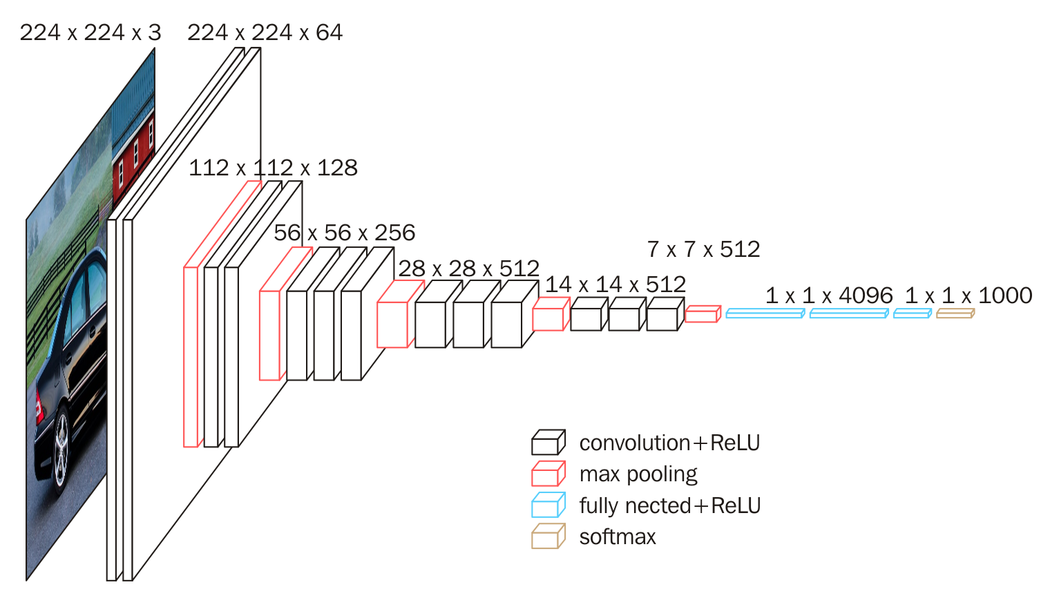
Here we implement the pre-trained VGG16 network. Instead of the final MaxPooling layer, we we add in a Global Average Pooling Layer at the end of the VGG16 architecture meaning the output of the network will be a single vector of numeric information rather than many arrays. We use “feature vector” to compare image similarity.
We pre-process our 300 base-set images, and then pass them through the VGG16 network to extract their feature vectors. We store these in an object for use when a search image is fed in.
We pass in a search image, apply the same preprocessing steps and again extract the feature vector.
We use Cosine Similarity to compare the search feature vector with all base-set feature vectors, returned the N smallest values. These represent our “most similar” images - the ones that would be returned to the customer.
Results
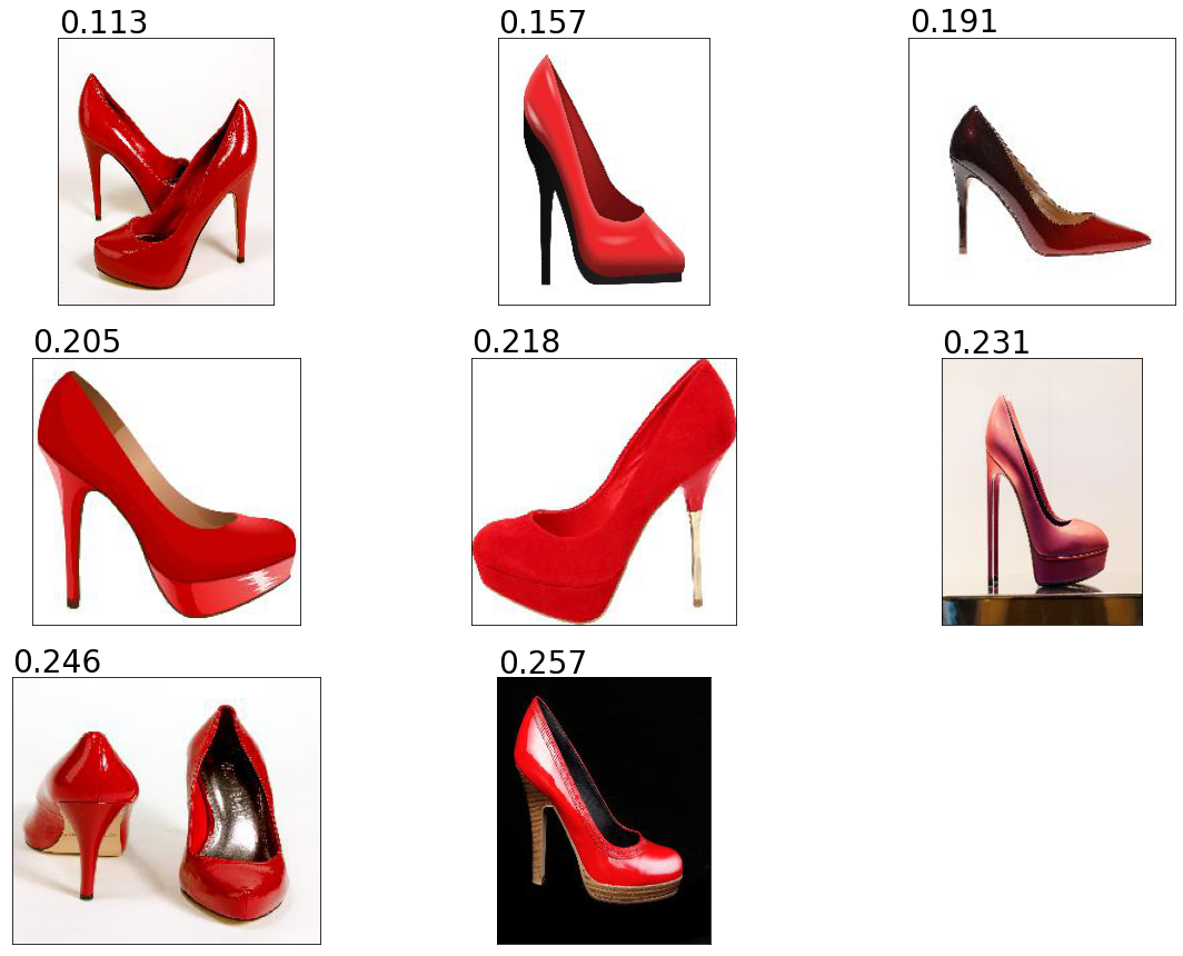
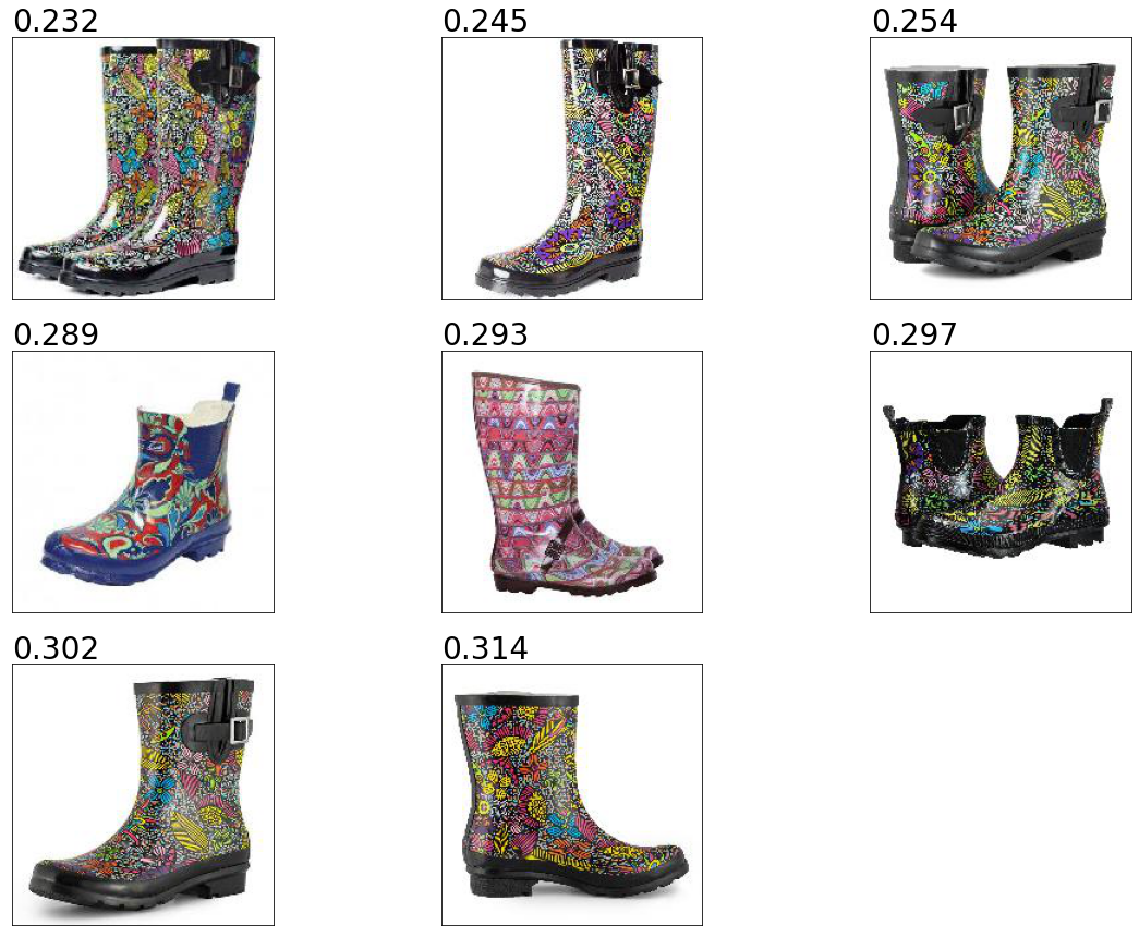
We test two different images, and plot the search results along with the cosine similarity scores. You can see these in the dedicated section below.
Discussion, Growth & Next Steps
The way we have coded this up is very much for the “proof of concept”. In practice we would definitely have the last section of the code (where we submit a search) isolated, and running from all of the saved objects that we need - we wouldn’t include it in a single script like we have here.
Also, rather than having to fit the Nearest Neighbours to our feature_vector_store each time a search is submitted, we could store that object as well.
When applying this in production, we also may want to code up a script that easily adds or removes images from the feature store. The products that are available in the clients store would be changing all the time, so we’d want a nice easy way to add new feature vectors to the feature_vector_store object - and also potentially a way to remove search results coming back if that product was out of stock, or no longer part of the suite of products that were sold.
Most likely, in production, this would just return a list of filepaths that the client’s website could then pull forward as required - the matplotlib code is just for us to see it in action manually!
This was tested only in one category, we would want to test on a broader array of categories - most likely having a saved network for each to avoid irrelevant predictions.
We only looked at Cosine Similarity here, it would be interesting to investigate other distance metrics.
It would be beneficial to come up with a way to quantify the quality of the search results. This could come from customer feedback, or from click-through rates on the site.
Here we utilised VGG16. It would be worthwhile testing other available pre-trained networks such as ResNet, Inception, and the DenseNet networks.
Sample Data Overview
For our proof on concept we are working in only one section of the client’s product base, women’s shoes.
We have been provided with images of the 300 shoes that are currently available to purchase. A random selection of 18 of these can be seen in the image below.

We will need to extract & capture the “features” of this base image set, and compare them to the “features” found in any given search image. The images with the closest match will be returned to the customer!
Transfer Learning Overview
Overview
Transfer Learning is an extremely powerful way for us to utilise pre-built, and pre-trained networks, and apply these in a clever way to solve our specific Deep Learning based tasks. It consists of taking features learned on one problem, and leveraging them on a new, similar problem!
For image based tasks this often means using all the the pre-learned features from a large network, so all of the convolutional filter values and feature maps, and instead of using it to predict what the network was originally designed for, piggybacking it, and training just the last part for some other task.
The hope is, that the features which have already been learned will be good enough to differentiate between our new classes, and we’ll save a whole lot of training time (and be able to utilise a network architecture that has potentially already been optimised).
For our Fruit Classification task we will be utilising a famous network known as VGG16. This was designed back in 2014, but even by todays standards is a fairly heft network. It was trained on the famous ImageNet dataset, with over a million images across one thousand different image classes. Everything from goldfish to cauliflowers to bottles of wine, to scuba divers!

The VGG16 network won the 2014 ImageNet competition, meaning that it predicted more accurately than any other model on that set of images (although this has now been surpassed).
If we can get our hands on the fully trained VGG16 model object, built to differentiate between all of those one thousand different image classes, the features that are contained in the layer prior to flattening will be very rich, and could be very useful for predicting all sorts of other images too without having to (a) re-train this entire architecture, which would be computationally, very expensive or (b) having to come up with our very own complex architecture, which we know can take a lot of trial and error to get right!
All the hard work has been done, we just want to “transfer” those “learnings” to our own problem space.
Nuanced Application
When using Transfer Learning for image classification tasks, we often import the architecture up to final Max Pooling layer, prior to flattening & the Dense Layers & Output Layer. We use the frozen parameter values from the bottom of the network, and then get instead of the final Max Pooling layer
With this approach, the final MaxPooling layer will be in the form of a number of pooled feature maps. For our task here however, we don’t want that. We instead want a single set of numbers to represent these features and thus we add in a Global Average Pooling Layer at the end of the VGG16 architecture meaning the output of the network will be a single array of numeric information rather than many arrays.
Setting Up VGG16
Keras makes the use of VGG16 very easy. We download the bottom of the VGG16 network (everything up to the Dense Layers) and then add a parameter to ensure that the final layer is not a Max Pooling Layer but instead a Global Max Pooling Layer
In the code below, we:
- Import the required packaages
- Set up the image parameters required for VGG16
- Load in VGG16 with Global Average Pooling
- Save the network architecture & weights for use in search engine
# import the required python libraries
from tensorflow.keras.models import Model, load_model
from tensorflow.keras.applications.vgg16 import VGG16, preprocess_input
from tensorflow.keras.preprocessing.image import load_img, img_to_array
import numpy as np
from os import listdir
from sklearn.neighbors import NearestNeighbors
import matplotlib.pyplot as plt
import pickle

# VGG16 image parameters
img_width = 224
img_height = 224
num_channels = 3

# load in & structure VGG16 network architecture (global pooling)
vgg = VGG16(input_shape = (img_width, img_height, num_channels), include_top = False, pooling = 'avg')
model = Model(inputs = vgg.input, outputs = vgg.layers[-1].output)

# save model file
model.save('models/vgg16_search_engine.h5')
The architecture can be seen below:
_________________________________________________________________
Layer (type)                 Output Shape              Param #
=================================================================
input_2 (InputLayer)         [(None, 224, 224, 3)]     0
_________________________________________________________________
block1_conv1 (Conv2D)        (None, 224, 224, 64)      1792
_________________________________________________________________
block1_conv2 (Conv2D)        (None, 224, 224, 64)      36928
_________________________________________________________________
block1_pool (MaxPooling2D)   (None, 112, 112, 64)      0
_________________________________________________________________
block2_conv1 (Conv2D)        (None, 112, 112, 128)     73856
_________________________________________________________________
block2_conv2 (Conv2D)        (None, 112, 112, 128)     147584
_________________________________________________________________
block2_pool (MaxPooling2D)   (None, 56, 56, 128)       0
_________________________________________________________________
block3_conv1 (Conv2D)        (None, 56, 56, 256)       295168
_________________________________________________________________
block3_conv2 (Conv2D)        (None, 56, 56, 256)       590080
_________________________________________________________________
block3_conv3 (Conv2D)        (None, 56, 56, 256)       590080
_________________________________________________________________
block3_pool (MaxPooling2D)   (None, 28, 28, 256)       0
_________________________________________________________________
block4_conv1 (Conv2D)        (None, 28, 28, 512)       1180160
_________________________________________________________________
block4_conv2 (Conv2D)        (None, 28, 28, 512)       2359808
_________________________________________________________________
block4_conv3 (Conv2D)        (None, 28, 28, 512)       2359808
_________________________________________________________________
block4_pool (MaxPooling2D)   (None, 14, 14, 512)       0
_________________________________________________________________
block5_conv1 (Conv2D)        (None, 14, 14, 512)       2359808
_________________________________________________________________
block5_conv2 (Conv2D)        (None, 14, 14, 512)       2359808
_________________________________________________________________
block5_conv3 (Conv2D)        (None, 14, 14, 512)       2359808
_________________________________________________________________
block5_pool (MaxPooling2D)   (None, 7, 7, 512)         0
_________________________________________________________________
global_average_pooling2d (Gl (None, 512)               0
=================================================================
Total params: 14,714,688
Trainable params: 14,714,688
Non-trainable params: 0
_________________________________________________________________
We used square brackets with - 1 and .output to denote that our output the one that we want is the final layer of our vgg object.
If we hadn’t added that last parameter of “pooling = avg” then the final layer would have been that MaxPoolingLayer of shape 7 by 7 by 512. Instead however, the Global Average Pooling logic was added, and this means we get that single array that is of size 512. In other words, all of the feature maps from that final Max Pooling layer are summarised down into one vector of 512 numbers, and for each image these numbers will represent it’s features. This feature vector is what we will be using to compare our base set of images, to any given search image to assess the similarity!
Image Preprocessing & Featurisation
Helper Functions
Here we create two useful functions, one for pre-processing images prior to entering the network, and the second for featurising the image, in other words passing the image through the VGG16 network and receiving the output, a single vector of 512 numeric values.
# image pre-processing function
def preprocess_image(filepath):

    image = load_img(filepath, target_size = (img_width, img_height))
    image = img_to_array(image)
    image = np.expand_dims(image, axis = 0)
    image = preprocess_input(image)

    return image

# image featurisation function
def featurise_image(image):

    feature_vector = model.predict(image)

    return feature_vector
The preprocess_image function does the following:
- Receives the filepath of an image
- Loads the image in
- Turns the image into an array
- Adds in the “batch” dimension for the array that Keras is expecting
- Applies the custom pre-processing logic for VGG16 that we imported from Keras
- Returns the image as an array
The featurise_image function does the following:
- Receives the image as an array
- Passes the array through the VGG16 architecture
- Returns the feature vector
Setup
In the code below, we:
- Specify the directory of the base-set of images
- Set up empty list to append our image filenames (for future lookup)
- Set up empty array to append our base-set feature vectors
# source directory for base images
source_dir = '/Users/praju/Desktop/DSI/Deep_Learning/Image Search Engine/data/'

# empty objects to append to
filename_store = []
feature_vector_store = np.empty((0,512))
Preprocess & Featurise Base-Set Images
We now want to preprocess & feature all 300 images in our base-set. To do this we execute a loop and apply the two functions we created earlier. For each image, we append the filename, and the feature vector to stores. We then save these stores, for future use when a search is executed.
# pass in & featurise base image set
for image in listdir(source_dir):

    print(image)

    # append image filename for future lookup
    filename_store.append(source_dir + image)

    # preprocess the image
    preprocessed_image = preprocess_image(source_dir + image)

    # extract the feature vector
    feature_vector = featurise_image(preprocessed_image)

    # append feature vector for similarity calculations
    feature_vector_store = np.append(feature_vector_store, feature_vector, axis = 0)

# save key objects for future use
pickle.dump(filename_store, open('models/filename_store.p', 'wb'))
pickle.dump(feature_vector_store, open('models/feature_vector_store.p', 'wb'))
Execute Search
With the base-set featurised, we can now run a search on a new image from a customer!
Setup
In the code below, we:
- Load in our VGG16 model
- Load in our filename store & feature vector store
- Specify the search image file
- Specify the number of search results we want
# load in required objects
model = load_model('/Users/praju/Desktop/DSI/Deep_Learning/Image Search Engine/models/vgg16_search_engine.h5', compile = False)
filename_store = pickle.load(open('/Users/praju/Desktop/DSI/Deep_Learning/Image Search Engine/models/filename_store.p', 'rb'))
feature_vector_store = pickle.load(open('/Users/praju/Desktop/DSI/Deep_Learning/Image Search Engine/models/feature_vector_store.p'', 'rb'))

# search parameters
search_results_n = 8
search_image = 'search_image_01.jpg'
The search image we are going to use for illustration here is below:

Preprocess & Featurise Search Image
Using the same helper functions, we apply the preprocessing & featurising logic to the search image - the output again being a vector containing 512 numeric values.
# preprocess & featurise search image
preprocessed_image = preprocess_image(search_image)
search_feature_vector = featurise_image(preprocessed_image)
Locate Most Similar Images Using Cosine Similarity
At this point, we have our search image existing as a 512 length feature vector, and we need to compare that feature vector to the feature vectors of all our base images.
When that is done, we need to understand which of those base image feature vectors are most like the feature vector of our search image, and more specifically, we need to return the eight most closely matched, as that is what we specified above.
To do this, we use the NearestNeighbors class from scikit-learn and we will apply the Cosine Distance metric to calculate the angle of difference between the feature vectors.
Cosine Distance essentially measures the angle between any two vectors, and it looks to see whether the two vectors are pointing in a similar direction or not. The more similar the direction the vectors are pointing, the smaller the angle between them in space and the more different the direction the LARGER the angle between them in space. This angle gives us our cosine distance score.
By calculating this score between our search image vector and each of our base image vectors, we can be returned the images with the eight lowest cosine scores - and these will be our eight most similar images, at least in terms of the feature vector representation that comes from our VGG16 network!
In the code below, we:
- Instantiate the Nearest Neighbours logic and specify our metric as Cosine Similarity
- Apply this to our feature_vector_store object (that contains a 512 length feature vector for each of our 300 base-set images)
- Pass in our search_feature_vector object into the fitted Nearest Neighbors object. This will find the eight nearest base feature vectors, and for each it will return (a) the cosine distance, and (b) the index of that feature vector from our feature_vector_store object.
- Convert the outputs from arrays to lists (for ease when plotting the results)
- Create a list of filenames for the eight most similar base-set images
# instantiate nearest neighbours logic
image_neighbours = NearestNeighbors(n_neighbors = search_results_n, metric = 'cosine')

# apply to our feature vector store
image_neighbours.fit(feature_vector_store)

# return search results for search image (distances & indices)
image_distances, image_indices = image_neighbours.kneighbors(search_feature_vector)

# convert closest image indices & distances to lists
image_indices = list(image_indices[0])
image_distances = list(image_distances[0])

# get list of filenames for search results
search_result_files = [filename_store[i] for i in image_indices]
Plot Search Results
We now have all of the information about the eight most similar images to our search image - let’s see how well it worked by plotting those images!
We plot them in order from most similar to least similar, and include the cosine distance score for reference (smaller is closer, or more similar)
# plot search results
plt.figure(figsize=(20,15))
for counter, result_file in enumerate(search_result_files):
    image = load_img(result_file)
    ax = plt.subplot(3, 3, counter+1)
    plt.imshow(image)
    plt.text(0, -5, round(image_distances[counter],3), fontsize=28)
    ax.get_xaxis().set_visible(False)
    ax.get_yaxis().set_visible(False)
plt.show()
The search image, and search results are below:
Search Image

Search Results

Very impressive results! From the 300 base-set images, these are the eight that have been deemed to be most similar!
Let’s take a look at a second search image…
search_image = 'search_image_02.jpg'
search_results_n = 8

preprocessed_image = preprocess_image(search_image)
search_feature_vector = featurise_image(preprocessed_image)

image_distances, image_indices = image_neighbours.kneighbors(search_feature_vector)

image_indices = list(image_indices[0])
image_distances = list(image_distances[0])

search_results_file = [filename_store[i] for i in image_indices]
# plot results

plt.figure(figsize=(20,15))
for counter, result_file in enumerate(search_results_file):
    image = load_img(result_file)
    ax = plt.subplot(3, 3, counter+1)
    plt.imshow(image)
    plt.text(0, -5, round(image_distances[counter],3), fontsize=28)
    ax.get_xaxis().set_visible(False)
    ax.get_yaxis().set_visible(False)
plt.show()
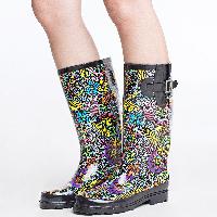
The search image, and search results are below:
Search Image

Search Results

Again, these have come out really well - the features from VGG16 combined with Cosine Similarity have done a great job!
Discussion, Growth & Next Steps
The way we have coded this up is very much for the “proof of concept”. In practice we would definitely have the last section of the code (where we submit a search) isolated, and running from all of the saved objects that we need - we wouldn’t include it in a single script like we have here.
Also, rather than having to fit the Nearest Neighbours to our feature_vector_store each time a search is submitted, we could store that object as well.
When applying this in production, we also may want to code up a script that easily adds or removes images from the feature store. The products that are available in the clients store would be changing all the time, so we’d want a nice easy way to add new feature vectors to the feature_vector_store object - and also potentially a way to remove search results coming back if that product was out of stock, or no longer part of the suite of products that were sold.
Most likely, in production, this would just return a list of filepaths that the client’s website could then pull forward as required - the matplotlib code is just for us to see it in action manually!
This was tested only in one category, we would want to test on a broader array of categories - most likely having a saved network for each to avoid irrelevant predictions.
We only looked at Cosine Similarity here, it would be interesting to investigate other distance metrics.
It would be beneficial to come up with a way to quantify the quality of the search results. This could come from customer feedback, or from click-through rates on the site.
Here we utilised VGG16. It would be worthwhile testing other available pre-trained networks such as ResNet, Inception, and the DenseNet networks.